LDA from scratch

The company where I work has a semi-regular, informal book club (for nerds – which we are). Recently, my supervisor has been giving talks on some papers which describe extensions of the Latent Dirichlet Allocation (LDA) topic modelling method. While I felt like I had a reasonable-enough high-level understanding, I didn’t feel like I knew the specifics well enough. If I had to do something where I’d have to make an Author-Recipient Topic Model [pdf], for example, I’d be lost (unless I found an existing R package, or so). I didn’t feel like I knew enough about the background probability, or about how to make a computer do anything given a model description and a bunch of data. So I started investigating things at this level, and presented what I had. There’s still plenty of gaps and uncertainty in my understanding, but I thought it’d be good to get notes together before I got too distracted by other things… So, the main goal with LDA is that you’re given a collection of documents (i.e., a corpus), and you’d like to determine a collection of topics that are represented in the documents (and in which proportion for each document), as well as the words which comprise each topic. You don’t know the topics ahead of time, and aim to just determine them based on the words you see in the document. There’s other approaches for accomplishing this, besides LDA; the most common seems to be Latent Semantic Analysis (LSA), which is very much like Principal Component Analysis (PCA), relying on the Singular Value Decomposition (SVD) of the so-called “term-document matrix”. But that’s all the topic of another day. Today, we’re sticking with LDA, which is a more probability-based approach. In this post, I’ll build up to LDA, starting with much similar models and questions. It’s been a while since I had a probability class, so I started with basics…

Coins

Suppose you’ve got a weighted coin, which has a probability $\phi$ of coming up heads. You flip the coin $N$ times, and obtain $n$ heads. What can you say about $\phi$ ? Well, the probability of obtaining $n$ heads is given by:

$\binom{N}{n}\phi^n(1-\phi)^{N-n}$ .

One way we can try to say something about $\phi$ is to ask which value of $\phi$ maximizes this expression. Calculus teachers, rejoice! Since the binomial coefficient in the front is constant with respect to $\phi$ , we can drop it, and simply try to maximize 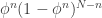$\phi^n(1-\phi^n)^{N-n}$ . Many students will, naturally, dive right in and differentiate this with product and chain rules. Students who have seen the tricks before (or are especially perceptive) will realize that the expression is maximized when its log is maximized, since log is monotonically increasing. So we aim to maximize $n\log(\phi)+(N-n)\log(1-\phi)$ , for $0<\phi<1$ . This derivative is easy to calculate, and has a single 0, at $n/N$ , which can be verified to be a local/absolute maximum.

So, that’s nice. And a lot of work to determine what everybody probably already knows. If you’ve got a biased coin that you flip 100 times, and obtain 75 heads and 25 tails, your guess probably should be that the sides are weighted 3 to 1 (i.e., that $\phi=.75$ ). Knowing that it’s all random to an extent, though, we aren’t certain of our answer. What we’re really like to know is the probability that $\phi$ is 0.75, versus, say, 0.72 (which could also certainly have generated the observed data).

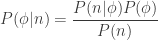
Well, this is what Bayes’ Theorem is for (or, at least, this is an application of it). We just calculated $P(n|\phi)$ , and want to, instead, calculate $P(\phi|n)$ . Bayes tells us we can do this via

$P(\phi|n) = \dfrac{P(n|\phi)P(\phi)}{P(n)}$ .

The denominator is the same as $\int_\phi P(n|\phi)P(\phi)\ d\phi$ (I’ll write $x$ ‘s below to either reduce or compound notational confusion, depending on your viewpoint). Substituting our expression for $P(n|\phi)$ , above, and cancelling the resulting binomial coefficients, we obtain

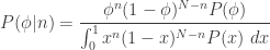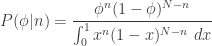
$P(\phi|n) = \dfrac{\phi^n(1-\phi)^{N-n}P(\phi)}{\int_0^1 x^n(1-x)^{N-n}P(x)\ dx}$ .

But there’s still unknown expressions in there! We still need to know $P(\phi)$ , in order to find $P(\phi|n)$ . That’s sorta frustrating. We could pick any probability distribution for $P(\phi)$ , how to we decide which to pick? Well, an easy choice would be the uniform distribution, because then we can just put 1 in the expression above in a few places, and obtain

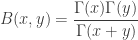
$P(\phi|n) = \dfrac{\phi^n(1-\phi)^{N-n}}{\int_0^1 x^n(1-x)^{N-n}\ dx}$ .

The denominator there has no $\phi$ s in it, and so is “just” a normalization constant (more on this in a moment). That is, $P(\phi|n)$ is basically given by $\phi^n(1-\phi)^{N-n}$ , once you divide by the integral of that expression over the domain (the interval from 0 to 1) so that you’ve got a probability distribution. The distribution we’ve obtained is called the Beta distribution, with parameters $n+1$ and $N-n+1$ (the “plus 1s” might become more sensible in a moment). With our 75 out of 100 example from before, this distribution is as follows:

The mode (not the mean) for this distribution is exactly what we calculated before, 75/100.

Now, something somewhat interesting just happened, without our trying much. We didn’t really have many good guesses for what the distribution of $P(\phi)$ , so we just picked the uniform distribution. It turns out that the uniform distribution is a special case of the Beta distribution, namely $B(x;1,1)$ . What’s noteworthy, if you’re into that sort of thing, is that we started with a “prior” guess for the distribution of $\phi$ of a certain form, $B(x;1,1)$ , and then we updated our beliefs about $\phi$ based on the data (the number of heads and tails flipped), and ended up with a “posterior” distribution for $\phi$ of the same “form”, $B(x;1+n,1+N-n)$ . This is sort of a happy accident, if you’re required to do this sort of Bayesian analysis by hand, apparently. It makes it easy to update again, if we flip the coin some more times. Suppose we flip several more times and see $H$ heads and $T$ tails. Well, we’d use our latest beliefs about $\phi$ , namely that it came from $B(x;1+n,1+N-n)$ , and then update that information as before. All that happened before was that we added the number of heads to the first parameter of the Beta distribution, and the number of tails to the second parameter, so we’d do that again, obtaining $B(x;1+n+H,1+N-n+T$ ). In fact, there’s no reason we’d have to cluster our flips into groups – with each flip we could update our Beta distribution parameters by simply adding 1 to the first parameter for a head, and to the second parameter for a tail. Oh, and the more formal description for what’s going on here, besides “happy accident”, is that the Beta distribution is the conjugate prior for the Binomial distribution.

This also suggests that we didn’t have to start with the uniform distribution, $B(x;1,1)$ , to have this happy accident occur. We could start with any $B(x;\alpha,\beta)$ , and then after observing $H$ heads and $T$ tails, we’d update our beliefs and say that $\phi$ came from $B(x;\alpha+H,\beta+T)$ . So maybe there’s a better choice for those initial parameters, $\alpha$ and $\beta$ ? In a very real sense, which we’ve already seen with this updating procedure, these parameters are our prior belief about the coin. If we’ve never flipped the coin at all, we’d sorta want to say that $\alpha$ and $\beta$ are 0, but the parameters of the Beta distribution are required to be positive. So we’d say we don’t really know, and choose a “weekly informative” prior, say 0.001 for both $\alpha$ and $\beta$ . The point of choosing such a small prior is that it lets the data have a strong governance on the shape of the distribution we get once we update our beliefs having seen some data. This is because $B(x;\alpha+n,\beta+N-n)$ is very similar to $B(x;n,N-n)$ if $\alpha$ and $\beta$ are small (relative to $n$ an $N-n$ ).

If you’d like to play around with actually running some code (and who doesn’t?), below is some R code I threw together. It simulates a sequence of flips of a weighted coin, and plots the progression of updates to our belief about $\phi$ as we run through the flips.

coinWeights <- c(.65,.35)

prior <- c(1,1)

numFlips <- 10

flips <- sample(1:2, numFlips, prob=coinWeights, replace=TRUE)
print(flips)

betaDist <- function(alphaBeta) {
  function(x) {
    dbeta(x, alphaBeta[1], alphaBeta[2])
  }
}

colors <- rainbow(numFlips)

plot(betaDist(prior), xlim=c(0,1), ylim=c(0,5), xlab="", ylab="")
for (n in 1:numFlips) {
  prior[flips[n]] <- prior[flips[n]] + 1
  func <- betaDist(prior)
  curve(func, from=0, to=1, add=TRUE, col=colors[n])
}

legend("topleft", legend=c("prior",paste("flip",c("H","T")[flips])), col=c("#000000",colors), lwd=1)

I ran it once, obtaining the following plot: So that’s fun. You might play with that code to get a sense of how choosing bad priors will make it take a while (many coin flips) before the posterior distribution matches the actual coin. Before moving on to more complicated models, I’d like to mention that calling the denominator we obtained when we applied Bayes’ Theorem, above, “just” a normalizing constant, above, is a dis-service. The denominator is a function of the parameters $\alpha$ and $\beta$ , as is called the Beta function. Right off the bat, Calculus teachers can again rejoice at the integral determining $B(.5,.5)$ :

$B(.5,.5)=\int_0^1 \dfrac{dx}{\sqrt{x}\sqrt{1-x}}=\cdots=\pi$ .

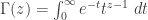
That integral’s doable by hand, and, unfortunately, an example of an exam question Calculus teachers probably would wet their pants over. But, better than simple tricks where goofy looking integrals “happen” to be related to circles (where did $\pi$ come from, there, anyway?), we also have

$B(x,y) = \dfrac{\Gamma(x)\Gamma(y)}{\Gamma(x+y)}$ ,

where

$\Gamma(z) = \int_0^{\infty} e^{-t}t^{z-1}\ dt$

is the analytic extension of $(z-1)!$ to the complex plane (our binomial coefficients from before seem to have been wrapped up into the normalizing constant, $B(\alpha,\beta)$ ). While I’m sure there’s no shortage of places you could read more about either the Beta or Gamma functions, I must say that I was enthralled with Artin’s book on the Gamma function. Delightful. Ok, moving on.

Dice

Let’s take a moment to slightly alter our notation, making it easy to extend to more dimensions (number of sides on the coin/die). Let’s write $\phi_1$ and $\phi_2$ for the probability of obtaining a head or tail on a single flip, respectively. Similarly, let’s write $n_1$ and $n_2$ for the number of observed heads and tails, respectively, with $N=n_1+n_2$ still the total number of flips. Just to double-check if you’re following, our original probability of obtaining this data from the parameter can now be written

$P(n|\phi) = \dfrac{N!}{n_1!n_2!}\phi_1^{n_1}\phi_2^{n_2}$ .

It’s probably now relatively easy to see how to generalize this. Suppose there are $V$ possible outcomes of our “coin” (/die/…), and that the probability of rolling side $i$ is given by $\phi_i$ (letting $\phi=(\phi_1,\ldots,\phi_2)$ ). Suppose we roll our die $N$ times, obtaining side $i$ a total of $n_i$ times (and letting $n=(n_1,\ldots,n_N)$ . Given just the sequence of rolls (and the number of sides), what can we say about $\phi$ ? The multi-dimensional generalization of the Beta distribution is the Dirichlet distribution. It takes parameters $\beta=(\beta_1,\ldots,\beta_V)$ and is defined over the points $x=(x_1,\ldots,x_V)$ having $0<x_i$ and $\sum_i x_i=1$ (i.e., $x$ lies on the hyper-triangle (simplex) spanned by the $V$ canonical unit vectors in $V$ -dimensional space). Its density function is

$D(x,\beta) = \dfrac{1}{B(\beta)}\prod_i x_i^{\beta_i-1}$ .

As before, we can treat $B(\beta)$ as “just” a normalization constant. One useful thing about the Dirichlet distribution is that it’s defined over a particular subset of $V$ -dimensional space – namely, the subset where the coordinates sum to 1 and are all positive. So if we draw a sample $\phi$ from $D(x;\beta)$ , then $\phi=(\phi_1,\ldots,\phi_V)$ can be thought of a discrete probability distribution defined on a set of size $V$ . More in line with the die example, a sample from $D(x;\beta)$ gives us weights for the sides of our die. The Beta distribution had the nice updating property described above – if we thought the parameters where $\alpha$ and $\beta$ and then we observed $n_H$ heads and $n_T$ tails, our new belief about the weight of the coin is described by parameters with values $\alpha+n_H$ and $\beta+n_T$ . The Dirichlet distribution updates just as nicely: If we previous thought the parameters were $\beta$ (a vector of length $V$ ), and then we observed counts $n$ ( $n_i$ the number of times we rolled side $i$ ), then our new parameters are simply $\beta+n$ . One of my goals, coming in to this learning project, was to actually figure out how to use OpenBUGS to do Bayesian analysis. Instead of doing the algebra by hand above to determine the posterior distributions (update our beliefs after we see some data), we’re supposed to be able to code up some model and provide it, with the data, to OpenBUGS, and have it return something like the answer. More specifically, BUGS, the Bayesian inference Using Gibbs Sampler, runs a Markov Chain Monte Carlo algorithm (presumably Gibbs sampling, based on the acronym), and returns to us draws from the posterior distribution. So even if we don’t know the analytic expression for the posterior, we can let OpenBUGS generate for us as many samples from the posterior as we’d like, and we can then address questions about the posterior distribution (e..g, what is the mean?) by way of the samples. I’d love, of course, to dig in to the mechanics of all this, but in the process of preparing my talk I found that another guy at work was already a few steps ahead of me down that road. So I’m going to let him tell me about it, which I very much look forward to. For now, my goal will simply be to figure out how to get OpenBUGS to answer the same question we’ve already done analytically in the case of a coin ( $V=2$ ): Given the sequence of rolls, what can it tell me about $\phi$ ? To start, let’s return to our apparently simple die-rolling procedure. What we have is a “generative model” for producing a data set. Specifically, we run through the following steps:

Choose a distribution of weights for sides of our die, by picking $\phi$ from $D(\beta)$ .
For each of iterations,
1. Roll the die, recording the side, $w_i$ , a sample from the categorical distribution $Cat(\phi)$ .

Having written what’s going on in this manner, we’re basically right at a description of the model in the BUGS language. What we’ve just written would get translated as:

model {
  phi[1:V] ~ ddirich(beta[])
  for (n in 1:N) {
    w[n] ~ dcat(phi[])
  }
}

(Your mileage may vary with ddirich versus ddirch.) However, this model isn’t quite complete enough. We haven’t said anything about $\beta$ in this model, but it certainly isn’t data we’ll be feeding in to the model (that’d be $w$ , the sequence of rolls). This is where I fall back on “wave the wand” – there’s still a fair amount of magic, for me, built into the priors when working with Bayesian inference. I’ll need to learn more about this, but for now, I’ll tell BUGS to use weakly informative priors (like we did with the coin). The complete model, then, is described to BUGS as:

model {
  phi[1:V] ~ ddirich(beta[])
  for (n in 1:N) {
    w[n] ~ dcat(phi[])
  }
  for (v in 1:V) {
    beta[v] <- 0.001
  }
}

But how does BUGS know what “V” and “N” and “w[n]” are? Well, we have to feed it the data. For this, I’ll let the R package rbugs do the hard work. I’ll work with relatively familiar R objects (which still surprise and frustrate me regularly), and let rbugs translate to and from OpenBUGS for me. The model above needs to be saved in a file, say ‘die.txt’. We can then use the following R code to play with this model and generate some pictures for us:

library(rbugs) # talk to OpenBUGS
library(coda) # MCMC utilities (mostly unused below)
library(gtools) # gives us ddirichlet

# set up parameters
# args <- strsplit("100 c(.7,.3) 1 5000 1000 .001", " ")[[1]]
args <- commandArgs(trailingOnly = TRUE)

# die parameters
n.rolls <- as.integer(args[1]) # 100
pre.phi <- eval(parse(text=args[2])) # c(.7,.3)
n.sides <- length(pre.phi) # 2 (calculated)

# mcmc parameters
n.chains <- as.integer(args[3]) # 1
n.iter <- as.integer(args[4]) # 5000
n.burnin <- as.integer(args[5]) # 1000
default.beta <- as.numeric(args[6]) # .001
# generate data
rolls <- sample(1:n.sides, n.rolls, prob = pre.phi, replace=TRUE)

# precalculate right answers
post.beta <- default.beta + tabulate(rolls)
post.phi.marginal <- cbind(post.beta, sum(post.beta)-post.beta) # phi[s] is Beta(beta[s]-1, sum(beta)-2)
post.phi.mean <- post.beta / sum(post.beta)
post.phi.mode <- (post.beta-1) / (sum(post.beta)-2)
post.phi.max <- apply(cbind(post.phi.mode, post.phi.marginal), 1, function(r) { dbeta(r[1], r[2], r[3]) })
# set up data to pass to bugs
die.data <- list(
 V = n.sides,
 N = n.rolls,
 w = rolls
 )
# generate initial values. rbugs doesn't seem to handle empty initial values well
inits <- function() {
 list(beta = rep(default.beta, n.sides))
}
# parameters to be saved, to compare with our algebraic calculations above
parameters <- c("phi")

# give us some samples! (make sure you have a directory 'tmp' under the pwd)
die.sim <- rbugs(die.data, inits, parameters, "die.txt",
 n.chains=n.chains, n.iter=n.iter, n.burnin=n.burnin,
 bugsWorkingDir="tmp", bugs="/usr/local/bin/OpenBUGS", cleanBugsWorkingDir=TRUE)
# coda provides some utilities for if you know enough about mcmc, which i don't
die.mcmc <- rbugs2coda(die.sim)
# die.mcmc is a list, with length = n.chains
# die.mcmc[[n]] has dimension c((n.iter-n.burnin), # variables)

base.filename = paste(args, collapse="_")

# save some stuff, in case you feel like poking at it
save(die.mcmc, args, rolls, file=paste(base.filename, 'RData', sep='.'))

# set up some drawing utilities
colors <- rainbow(n.sides)
xlim <- c(-.05, max(c(pre.phi, max(post.phi.mean)))+.1)
ylim <- c(-.05, 1.05)

draw.mean.line <- function(x, y, col, lty) {
 lines(c(x,x), ylim, col=col, lty=lty)
 text(x, y, col=col, labels=sprintf("%.03f", x))
}

draw.samples.density <- function(chains, varname, col, lty) {
 samples <- chains[[1]][,varname]
 den <- density(samples)
 den$y <- den$y / max(den$y)
 lines(den, col=col, lty=lty)
 draw.mean.line(mean(samples), -.03, col, lty)
}

# draw the sample distributions, as well as the given distrbution
png(paste(base.filename, 'png', sep='.'), width=1000, height=800)
plot(NULL, xlim=xlim, ylim=ylim, xlab=NA, ylab=NA, main=base.filename)

for (idx in 1:n.sides) {
 # actual
 draw.samples.density(die.mcmc, paste("phi[",idx,"]", sep=""), colors[idx], 1)

# show the original chosen values for phi
 draw.mean.line(pre.phi[idx], 1.03, colors[idx], 4)

# plot the algebraic answer, scaled to have max 1
 curve(dbeta(x, post.phi.marginal[idx,1], post.phi.marginal[idx,2]) / post.phi.max[idx], lty=2, add=TRUE, from=0, to=xlim[2])
 text(post.phi.mean[idx], .5+.1*(n.sides/2)-.1*(idx), labels=sprintf("%.03f",post.phi.mean[idx]))
}
legend("topleft", col=colors, lty=1, legend=paste("[",1:n.sides,"]",sep=""), title="phi")

dev.off()

For grins, here’s the output of one of my runs: Can you work out how many rolls there were for each of the sides? Having a script like this makes it pretty easy to investigate some questions:

What happens if I have more rolls ( $N$ )? Fewer?
If I pick a bad prior (e.g., a $\beta$ with large values), what happens to the output? How can it be compensated for? To what extent?
What about those iterations and burnin parameters? And just how does BUGS give us these samples anyway? Another day…

Basically there’s a bunch of knobs to twiddle, and all sorts of fun can be had. But let’s see if we can actually get closer to LDA, shall we?

Hierarchical Dice

Let’s add a layer of indirection. Suppose we’ve got a collection of weighted dice ( $K$ of them), each with the same number of sides (still $V$ ), but each possibly weighted differently. Let’s also suppose we’ve got a separate weighted die with $K$ faces. Let’s call the die with $K$ sides the T-die, and the other dice will be the W-dice. Now instead of just rolling a single die repeatedly, we’ll repeatedly (still $N$ times) do the following:

Roll the T-die to decide which of the W-dice to roll.
Roll the appropriate W-die, and record the result.

Given the sequence of rolls (where a ‘1’ on one W-die is not distinguished from a ‘1’ on another W-die), along with $K,V,N$ , can we determine the weights of the T-die and W-dice? Naturally, we should expect that this will go better when $N$ is relatively large. Perhaps someday I’ll come back and fill in the algebra here, but for now let’s just see what we need to do in order to get OpenBUGS to help us out again. First off, we don’t know the weights of the T-die, and we want it to help us learn those. Let’s say they are $\theta_1,\ldots,\theta_K$ , or more concisely the vector $\theta$ . As before, this is a discrete probability distribution, and we’ve seen that a sample from a Dirichlet gives us such a beast. So it seems sensible to suppose that $\theta$ is chosen from some $Dir(x;\alpha)$ , for some hyper-parameter $\alpha$ (a $K$ -dimensional vector). As before, we’ll feed in weakly informative priors. Next up, we have the weights of the sides on each of the W-dice. Before, we only had one such die, and the weights of its sides were $\phi$ . So let’s stick with $\phi$ for these weights, but now it must become a matrix – specifically, it has to be a $K\times V$ matrix. Each row in this matrix is, again, a probability distribution, so we’ll assume $\phi_{i,\bullet}$ is chosen from some $Dir(x;\beta)$ , where $\beta$ is a single $V$ -dimensional vector. All together, then, the model looks like:

model {
  theta[1:K] ~ ddirich(alpha[])
  for (k in 1:K) {
    phi[k,1:V] ~ ddirich(beta[])
  }
  for (n in 1:N) {
    z[n] ~ dcat(theta[])
    w[n] ~ dcat(phi[z[n],])
  }
  for (k in 1:K) {
    alpha[k] <- .1
  }
  for (v in 1:V) {
   beta[v] <- .001
  }
}

There’s enough parameters around that I haven’t bothered trying to make a nice clear picture of the outputs of this. The changes necessary to simply run the thing, beginning with the R code above, are pretty minimal – take in a couple extra parameters, generate samples via the two-step process, and figure out what you’d like to do with the outputs, and you’re set. Of course, I haven’t worked out the algebraically correct answers here… But we’re now knocking on the door of

LDA

Instead of only having a single T-die, suppose you’ve got several ( $M$ , say). After your $N$ rolls using your first T-die, and their tabulation to $n$ , from before, you decide to repeat the process with the second T-die (roll it $N$ times, each time rolling the appropriate W-die and recording the answer), and then go through it all again with the third T-die, and so on. Each time you use the same set of W-dice… Ok, the dice viewpoint has gotten stretched far too thin. Who would have that many weighted dice, and be interested in all those rolls anyway? Let’s translate over to document collections. Suppose you’ve got a collection of $M$ documents (a “corpus”, in the parlance of our time), each with $N$ words (for notational convenience, there’s no reason they all really need to have the same length). Suppose, moreover, that each document is actually a blend of any of $K$ topics, and that each document pertains to each topic in different proportions (weights of your T-dice). Finally, suppose each topic is represented by any of $V$ words (finally, $V$ for “vocabulary”!), and that the different topics have different weights for the $V$ words (your W-dice all had potentially different weights for their sides, but all had the same number of sides). Given only the word sequences for the documents, the job of LDA is to uncover the topic distribution for each document (the weights of the sides of the associated T-die) as well as the word frequency distributions corresponding to each topic (the weights of the various W-dice). But really, this is only a step or two harder than uncovering the weights of a biased coin, which we began with. There’s sort of an assumption floating around in here that the order of words in documents doesn’t much matter. The brief look I had the original LDA paper [pdf] has me thinking that this has nice theoretical consequences concerning the form of the model for generating documents. Basically, under our assumption that documents are generated by repeatedly picking a topic (rolling a T-die) and then picking a word based on the word weights for that topic (rolling the appropriate W-die), the parameters have to be as described as in the following BUGS model:

model {
  for (k in 1:K) {
    phi[k,1:V] ~ ddirich(beta[]) # weights of W-die k
  }
  for (d in 1:M) {
    theta[d,1:K] ~ ddirich(alpha[]) # weights of T-die d
    for (n in 1:N) {
      z[d,n] ~ dcat(theta[d,])    # the n-th T-die roll for document d (choose a topic)
      w[d,n] ~ dcat(phi[z[d,n],]) # the n-th W-die roll for document d (choose a word from topic z[d,n])
    }
  }
}

I took the priors out, above; mostly I still feel like they’re a gap in my understanding. But whatever, good enough. It’s natural at this point to wonder how you’d take the word order into account anyway; I haven’t looked into it much, but there’s at least one paper [pdf] on the subject. One might also wonder how to to determine the number of topics if that constant ( $K$ ) isn’t given to you with the word count tabulations. Again, this has been addressed [pdf], though I haven’t dug into it a whole lot. And let’s not forget, let’s not forget, that I still have basically no idea how or why Gibbs sampling (and/or other MCMC methods – Metropolis-Hastings, I’m looking at you) works. Finally, I was honestly a little surprised to find that the OpenBUGS model above, and the R script I coded up to use it, took something like 8 hours on sample data I generated to throw at it (maybe 1000 words, 3 documents, 2 topics, or so). I then looked at the lda package in R, manipulated my sample data so I could feed it to that, and got answers out in about a second. Clearly there’s something else going on there. My investigations so far have me thinking the difference is probably described in this paper, but it, along with everything else I’ve just mentioned, is still in the “todo” pile. So, more questions than answers, though I feel like I answered a few questions for myself in all of this. It’s probably some sort of life lesson that learning one thing just opens up the doors for not knowing a whole bunch more, or something. Hopefully I’ll keep chipping away on these or related topics (or, at least, something interesting). And maybe I’ll just find the energy to write about it, to help point out all the things I don’t understand. Anyway, thanks for coming with me on this. Sorry it took me so long, and left so many questions. In addition to the links above, I found this paper helpful/interesting.

Update 2015071: Corrected variable of integration in formula for $\Gamma(z)$, thanks to comment by Joel Nothman.

This entry was posted on June 13, 2012 at 7:03 pm and is filed under Play. You can follow any responses to this entry through the RSS 2.0 feed. You can leave a response, or trackback from your own site.

4 Responses to “LDA from scratch”

Mathblogging.org Weekly Picks « Mathblogging.org — the Blog Says:
June 20, 2012 at 9:53 pm | Reply
[…] ∑idiot’s Blog gives you Latent Dirichlet Allocation from scratch. […]
ranga Says:
November 24, 2012 at 11:57 pm | Reply
This is really really helpful Nick. Worth reading it b’coz it’s well written and nice flow of arguments.
You made my day.
Thanks again for your time Nick.
Joel Nothman Says:
July 6, 2015 at 2:45 am | Reply
Your definition of Gamma should be corrected: it should be dt, not dz.
- sumidiot Says:
  July 11, 2015 at 2:03 pm | Reply
  Thanks! Corrected.

∑idiot's Blog

LDA from scratch

Coins

Dice

Hierarchical Dice

LDA

4 Responses to “LDA from scratch”

Leave a comment Cancel reply

∑idiot's Blog

LDA from scratch

Coins

Dice

Hierarchical Dice

LDA

Share this:

Related

4 Responses to “LDA from scratch”

Leave a comment Cancel reply